
Table of contents
* Preliminary summary
* The electromagnetic field solution
* Electric Power Line Equation
* Matlab drawing
Supplement: Equation of lines of force
Collapse
Preliminary summary
Xu Damiao, who studies science: the solution and application of D’Alembert’s equation in the electromagnetic field
10 likes · 2 comments on the article The vector bit distribution generated by the unit dipole in space has been obtained above: ps: The element dipole changes sinusoidally, using the phasor method to solve
The distribution of the electromagnetic field in space can be further solved by using the vector bit A: This paper analyzes the electromagnetic radiation produced by the unit dipole on this basis. Second, the electromagnetic field solution The vector bit A is decomposed into spherical coordinates along the ez direction of the Cartesian coordinate system, and the components are written: Solve for the magnetic field B in spherical coordinates: Then calculate the electric field E: 1*) Find the divergence in the spherical coordinate system—— 2*) Find the gradient in the spherical coordinate system—— 3*) Substitute into the expression for the electric field E (using β=ωμε)—— To sum up, write the phasors of the electric field E and magnetic field H in component form: So far, the electromagnetic field distribution generated by the unit dipole antenna in space is obtained.
Electric Power
Line Equation
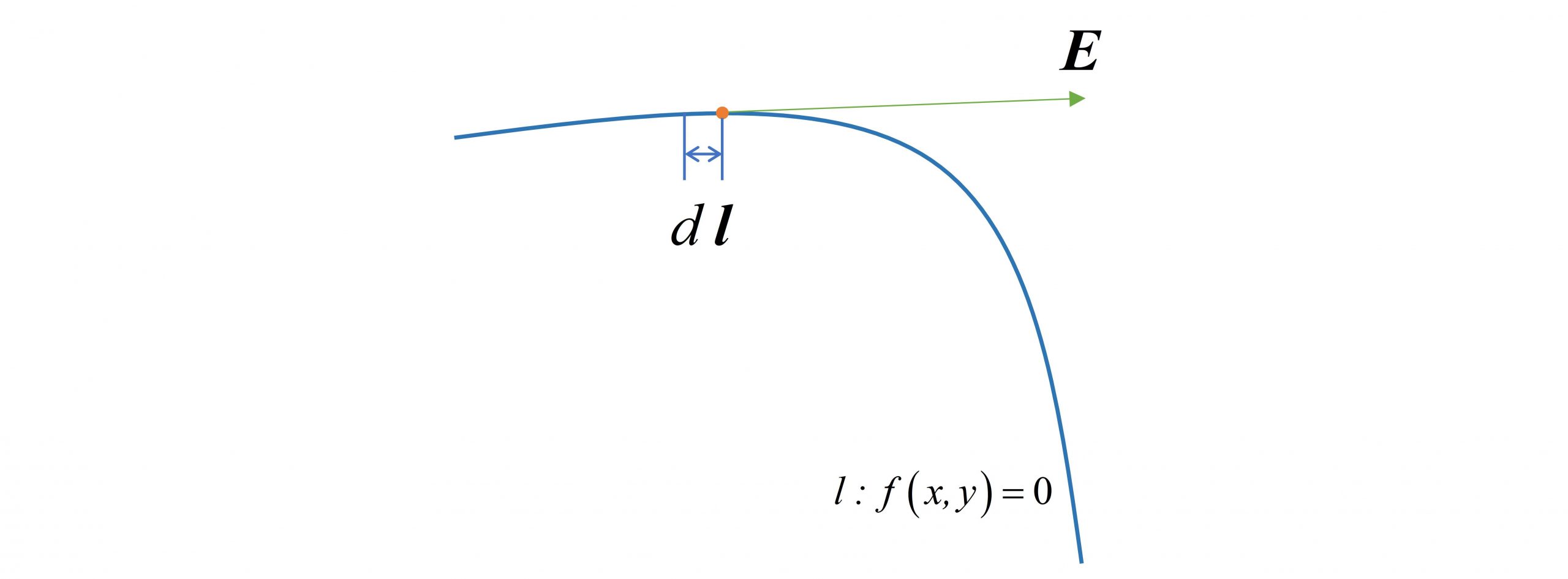
In the second section, the magnitude and direction of the electric field intensity E at any point in the space are obtained. In order to describe the electric field distribution more vividly, it is necessary to solve the electric force line equation. The electric force line is a cluster of curves, and the tangent direction of each point on the curve is the direction of the electric field intensity at that point, as shown in the figure below: In order to describe the characteristics of the electric power line, take a length element dl=(dx,dy,dz) on the line, which is in the same direction as E, then satisfy: In addition, the characteristics of the electric force line are described in the spherical coordinate system as: Then get the differential equation that the electric force line satisfies, and solve this equation to get the electric force line equation. The visualization of the electromagnetic field can be easily realized by using matlab to draw the cluster of electric force lines. Four, matlab drawing
Since the electric field component in the electric force line differential equation is the actual value of the electric field, it is necessary to transform the electric field phasor expression obtained in the second section into an instantaneous value expression: Substitute into the power line differential equation: Simplification: Integrating the left and right sides of the equation, we can get the power line equation, where: Therefore, the result of the solution is: Among them, C is an integral constant, and each value of C corresponds to a power line, and a cluster of power lines can be obtained by taking a set of C values. Draw the lines of force generated in space by an elemental dipole antenna as follows: When drawing, take a certain set of C values, and draw the power line cluster corresponding to this set of C values at each moment
analyze– It can be seen that the power line is generated by the unit dipole antenna. At the same time, due to the mutual excitation of the electric field and the magnetic field, the power line breaks away from the antenna and propagates outwards beyond a certain distance. This is the principle of the radiation of the unit dipole antenna. Supplement: Equation of lines of force
Like the line of force, the line of force is a set of equations describing the magnetic field, and the tangent direction of each point on the curve is the direction of the magnetic field strength at that point. The magnetic field line equation satisfies the condition: In addition, the magnetic field line equation can also be derived from the vector position A: It can be seen from the second section that in this example, the magnetic field strength is along the eϕ direction of the spherical coordinate system, that is, Hz=0, and the magnetic force line equation satisfies the condition: Formula 4-1
The vector bit A is along the z-axis direction, Ax=0, Ay=0, when solving the magnetic induction: get: Substitute into the constraint condition (4-1) of the magnetic force line equation: That is, the rate of change of Az on the magnetic force line is zero, so the magnetic force line in this example is equal to the A line. Write the equation of the lines of force in terms of the expression for the vector position A: Each group of C values corresponds to a cluster of magnetic force lines, as follows, draw the magnetic force lines generated by the unit dipole antenna in space: ps: In the spherical coordinate system, the electric field E is distributed along the meridian direction, so the electric field lines of the xoz plane are drawn when drawing; the magnetic field H is distributed along the latitude direction, and the electric field lines of the xoy plane are drawn when drawing. In addition, give more visualization solutions—— 1*) Use the z-axis to represent the magnitude of the magnetic field strength, and draw the magnetic field distribution on the xoy plane: 2*) In this example, electromagnetic waves propagate in the form of spherical waves, so a radial direction can be used to demonstrate the changes of electric and magnetic fields: Taking the y-axis direction, the x-axis represents the magnitude and direction of the magnetic field, the y-axis represents the magnitude and direction of the electric field, and electromagnetic waves propagate along the y-axis direction: It can be seen that near the origin, that is, the near-field region of the unit dipole, the electric field lags behind the change of the magnetic field, while in the far-field region, the electric field and the magnetic field are in phase, which is consistent with common theoretical analysis. Draw the electromagnetic field change in the far field area in this direction separately, and you can see the propagation characteristics of electromagnetic waves

